
Why a laboratory needs a common 10 MHz and 1 pps
A frequency counter is never more accurate than its time base, and neither is the output of a signal generator. When two instruments each run on their own OCXO, the error the counter reads is really the difference between two oscillators and you cannot tell which side is off. Connect the external reference input of every instrument to the same 10 MHz source and the problem disappears: there is no relative error left between instruments, only the error of the reference itself against the true value, and that is a single number that can be calibrated and recorded.
The 10 MHz solves frequency and phase; the 1 pps solves time. Any measurement that has to say at what instant something happened, such as event time stamping, multi-site synchronization, IRIG-B time code or time alignment in a communication system, needs a seconds pulse aligned to UTC. The FTR-210R provides 5×10 MHz, 1×5 MHz and 1×1 pps in its standard configuration, with options adding 2×100 MHz plus 2×10 MHz and programmable pulses from 0.5 Hz to 100 MHz including IRIG-B DCLS, so that one unit acts as both the frequency and the time house reference.
There is a second benefit: calibration effort is concentrated in one place. Instead of sending the time base of every instrument out for calibration, you maintain traceability of the reference, and every instrument connected to it benefits on the frequency item (other items on the instrument still need calibration to their own specification).
What traceability to UTC actually means
Traceability is not a synonym for accurate. It is a chain that can be followed: your reference has been compared against a higher order standard, that standard against a national standard, and the national standard takes part in the international comparisons that form UTC. Every link needs a comparison method, a comparison result and an uncertainty, and all of it has to be recorded. Miss the documentation at any link and the chain is broken, however stable the instrument itself may be.
GNSS is the most practical route to traceability in a laboratory because the time scale of a satellite navigation system is itself monitored and compared continuously by national timing laboratories, so a receiver in lock extends that chain into your equipment room. The 1 pps of the FTR-210R is accurate to UTC to better than 10 ns rms, and the CNT-104R with the optional GNSS module reaches a frequency calibration accuracy of 1×10⁻¹² on a 24 hour average with time calibration uncertainty better than 10 ns rms to UTC. Those figures are the uncertainty of the last link in the chain.
Locked to GNSS and holding evidence of traceability are two different things, though. What an assessor wants to see is documentation. Option 220 on the FTR-210R is a documenting frequency comparator that runs independently of the disciplining loop, comparing the internal rubidium clock against GNSS continuously and generating a record. What you hand over is therefore not a front panel that says locked, but a set of comparison data over time. That is what built-in traceable calibration means in practice.
Choosing between a GNSS-disciplined rubidium and a standalone reference
A GNSS-disciplined rubidium clock uses satellite time to steer a rubidium oscillator over the long term: short-term stability comes from the rubidium, long-term accuracy from GNSS, and the two complement each other. When the satellite signal is interrupted the unit enters holdover and the rubidium is on its own. Typical holdover drift on the FTR-210R is 1 µs per 24 hours, and the aging rate in manual holdover is better than 5×10⁻¹¹ per month. A brief antenna outage therefore does not immediately affect frequency work, but the time output (1 pps) walks away gradually for as long as the outage lasts.
A standalone reference does not depend on satellites at all. The 6688 is built around an OCXO with a calibration uncertainty of 5×10⁻⁹ (+23 ±3 °C), an aging rate of 3×10⁻⁹/month and 2×10⁻⁸/year, short-term stability of ADEV 5×10⁻¹² (τ=1 s / 10 s), and it reaches 5×10⁻¹⁰ after a 10 minute warm-up. The 6689 uses a rubidium clock instead, with a calibration uncertainty of 5×10⁻¹¹, an aging rate of 5×10⁻¹¹/month and 1×10⁻⁹ over 10 years, ADEV of 3×10⁻¹¹ / 1×10⁻¹¹, lock in 5.4 minutes and 4×10⁻¹⁰ after 10.6 minutes. Power draw differs too: the 6688 runs continuously below 7 W, the 6689 below 30 W.
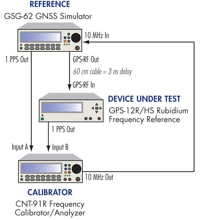
When is a standalone reference the right answer? Wherever a GNSS antenna cannot be installed, such as EMC shielded rooms and anechoic chambers, ships and submarines, tunnels and underground facilities, and sites where an external radio signal raises a security concern, and on production lines that need frequency only and never have to align to UTC time. The price is that traceability becomes a human task: a standalone reference has to be compared against a traceable reference on a schedule, for instance by taking it to a laboratory that has an FTR-210R, or by bringing in a calibrated counter with a built-in rubidium clock such as the CNT-91R or CNT-104R. The interval follows from the aging rate and your acceptance limit. The 6688 ages about 2×10⁻⁸ in a year, so if the acceptance limit is 1×10⁻⁷ then annual comparison is a reasonable starting point; the 6689 ages more than an order of magnitude more slowly and the interval can be longer, but the records still have to exist.
Many laboratories end up with two tiers: an FTR-210R as the traceable primary reference, and a 6688 or 6689 as a local reference in the shielded room or on the production floor, compared back to the primary on a schedule. That keeps traceability without having to bring a GNSS signal into every room.
Distributing the reference to many instruments
The output count of the reference is a hard limit. The FTR-210R has 5×10 MHz, 1×5 MHz and 1×1 pps as standard and expands to at most 11 outputs; the 6688/6689 provide, depending on model, 5 ports (668X/011) or 10 ports (668X/021) of 10 MHz sine plus 1 port of 5 MHz at an output level of 0.5 Vrms into 50 Ω. Give every instrument its own port in a star topology, and do not use a T connector to daisy-chain one port to several instruments: the reflections caused by the impedance mismatch leave each instrument seeing a different phase and level, and they make fault finding much harder.
Once the instrument count exceeds the port count, or the signal has to reach another room or another building, you need a distribution amplifier. The FDA-301 is a point-to-multipoint reference frequency and time synchronization distribution amplifier: sine distribution from 100 kHz to 60 MHz (10 MHz by default), pulse distribution with a bandwidth up to 20 MHz (suitable for 1 pps and IRIG-B DCLS), coax modules to a maximum of 12 ports (3 × 4), fiber modules to a maximum of 18 ports (3 × 6), and fiber runs up to 2 km. The dual primary/secondary input switches automatically, so you can feed one input from the primary reference and the other from a backup and the instruments never lose signal when the primary fails.
Distance is not the only reason to run fiber. Fiber does not conduct, so it isolates ground potential differences and lightning between two locations, and it does not carry RF noise from outside a shielded room into it, which matters particularly for EMC laboratories. Also keep cable delay in mind for the 1 pps: coax adds a few ns per meter and 2 km of fiber adds delay in the microsecond range, so a time comparison has to measure that delay and subtract it in the record, otherwise traceability at the 10 ns level is meaningless.
What to check when the GNSS antenna is obstructed
First establish whether the problem is the signal or the equipment: look at whether the satellite count and signal quality at the receiver have dropped sharply, whether the unit has gone from locked to holdover, and when the state changed. An antenna whose sky view is blocked by a new building, a construction crane or rooftop equipment usually shows as a satellite count falling day by day; a cable, surge arrester or connector that has taken in water usually shows as everything disappearing at once. The antenna should have a clear view of the sky, sit away from other transmitting antennas, and its cable length and loss should be within what the receiver allows.
Once the unit is in holdover, use the drift specification to estimate the effect. The typical FTR-210R figure of 1 µs per 24 hours means that after a day of outage the 1 pps may be roughly 1 µs away from UTC, while on the frequency side the aging rate in manual holdover is better than 5×10⁻¹¹ per month, which has limited effect on most frequency calibration work. Frequency work can therefore usually continue during an outage, but calibration of time against UTC should be suspended, and the start and end of the holdover period noted in the record.
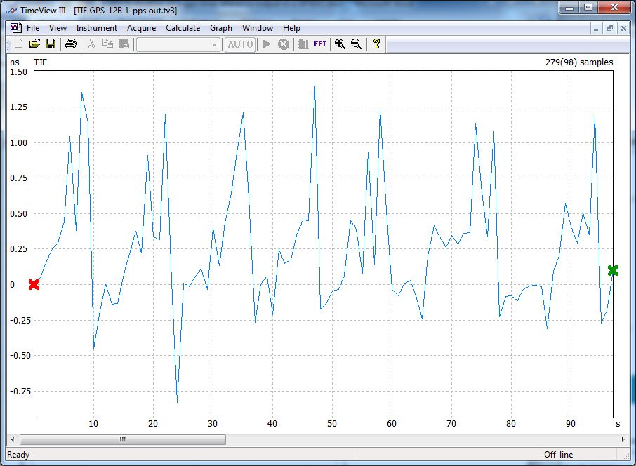
Do not treat the system as normal the moment lock returns. Check whether the 1 pps jumped when the receiver relocked, check whether the Option 220 comparator record shows how far the rubidium actually drifted during the outage, and keep that record. If outages are frequent, the thing to address is the antenna location, or a 6689 installed as a local reference in the critical areas so that they do not depend on satellites at all.
How to record and document the calibration
The documentation has to answer three questions: why the reference itself can be trusted, what the relationship is between each instrument and the reference, and how often that relationship is confirmed. The first is the traceability evidence for the reference: the Option 220 comparator record on the FTR-210R, the GNSS lock status log, and the periodic comparison reports between standalone references (6688/6689) and the primary. Those reports need a date, the ambient temperature (the calibration uncertainty of the 6688/6689 is defined at +23 ±3 °C), the comparison method and the uncertainty.
The second is the comparison of each instrument against the reference. The most direct method is to measure the 10 MHz output of every instrument with a calibrated counter: the CNT-91R offers 12 digits/s of frequency resolution and a built-in rubidium clock, and the optional measurement input on the FTR-210R (DC to 400 MHz, 12 to 13 digits at a 1 second gate) lets the comparison be done at the reference itself without moving another instrument into place. Record the frequency offset, the gate time, the number of measurements and the standard deviation, and state in the report which reference the counter itself was connected to.
The third is the interval and the acceptance limit. Derive the comparison interval from the aging rate in the specification and your own acceptance limit, and write into the procedure what happens when the limit is exceeded. Time and frequency measurement has the advantage of being almost fully automatable: a counter can log for long periods and the built-in web server of the FTR-210R can be read remotely, and collecting those logs centrally is far more reliable than reconstructing records after the fact. For help choosing the counter used in the comparison, see "Frequency Counter Selection Guide: Resolution, Channels and Time Base" Frequency Counter Selection Guide: Resolution, Channels and Time Base.